Demo applications DX-RT 3.2.0
DEEPX provides demo applications through the dx-app repository. These applications are included in the pre-built images provided by Embedded Artists, and can also be built into custom Yocto images by including the meta-ea-dx Yocto layer.
The way to run applications is version dependant. To check which version is being used, run dxrt-cli -s on target. The DXRT version shown on the first line like this. For 3.2.0 it looks like this:
DXRT v3.2.0
=======================================================
 * Device 0: M1, Accelerator type
---------------------   Version   ---------------------
This page is only for version 3.2.0 and later. For older versions visit Demo applications up to DX-RT 3.1.0.
All examples on this page were executed on RZ/G3E hardware running on an official build available on sw.embeddedartists.com. Note that the official builds does not include the Renesas proprietary graphics and codec drivers so the profiling data below is quite low. See instructions on the wiki, specifically Add Proprietary Packages for information about adding the support.
Models and resources
To run the demo applications, compiled DNNX models as well as additional resources - such as sample videos and images - are required. These resources are not installed by default and must be downloaded separately by following the steps below.
- Download and unpack models.
The compiled models are downloaded from the DEEPX resource directory and unpacked into the directory: assets/models.
There are version dependencies between DEEPX software components, as described in the Version compatibility section. The example below downloads models that are compatible with dx-app version 2.2.0.
wget https://sdk.deepx.ai/res/models/models-2_2_0.tar.gz
mkdir -p assets/models
tar -xvf models-2_2_0.tar.gz -C assets/models/
- Download and unpack sample videos
Sample video files are downloaded from the DEEPX resource directory and unpacked into the directory: assets/videos.
wget https://sdk.deepx.ai/res/video/sample_videos.tar.gz
mkdir -p assets/videos
tar -xvf sample_videos.tar.gz -C assets/videos/
- Download sample images
Sample image files are downloaded from the dx-app GitHub repository and stored in the directory: assets/images.
mkdir -p assets/images
wget -P assets/images/ https://raw.githubusercontent.com/DEEPX-AI/dx_app/refs/heads/main/sample/ILSVRC2012/1.jpeg
wget -P assets/images/ https://raw.githubusercontent.com/DEEPX-AI/dx_app/refs/heads/main/sample/img/7.jpg
wget -P assets/images/ https://raw.githubusercontent.com/DEEPX-AI/dx_app/refs/heads/main/sample/img/8.jpg
About Examples
In version 3.2.0 of DX_RT there was a major overhaul of the demo applications. According to the release notes
To improve user understanding, separated the previously integrated example code by Task (classification, object detection, segmentation, face recognition, pose estimation) / Model (EfficientNet, YOLO, YOLO_PPU, SCRFD, ...) / Inference method (sync, async) / Post-processing (pure python, pybind)
As a result, instead of having yolo, segmentation, classification and pose there are now the following:
/usr/bin/deeplabv3_async           /usr/bin/yolov5_async
/usr/bin/deeplabv3_sync            /usr/bin/yolov5_ppu_async
/usr/bin/efficientnet_async        /usr/bin/yolov5_ppu_sync
/usr/bin/efficientnet_sync         /usr/bin/yolov5_sync
/usr/bin/scrfd_async               /usr/bin/yolov5face_async
/usr/bin/scrfd_ppu_async           /usr/bin/yolov5face_sync
/usr/bin/scrfd_ppu_sync            /usr/bin/yolov5pose_async
/usr/bin/scrfd_sync                /usr/bin/yolov5pose_ppu_async
/usr/bin/yolov10_async             /usr/bin/yolov5pose_ppu_sync
/usr/bin/yolov10_sync              /usr/bin/yolov5pose_sync
/usr/bin/yolov11_async             /usr/bin/yolov7_async
/usr/bin/yolov11_sync              /usr/bin/yolov7_ppu_async
/usr/bin/yolov12_async             /usr/bin/yolov7_ppu_sync
/usr/bin/yolov12_sync              /usr/bin/yolov7_sync
/usr/bin/yolov26_async             /usr/bin/yolov7_x_deeplabv3_async
/usr/bin/yolov26_sync              /usr/bin/yolov7_x_deeplabv3_sync
/usr/bin/yolov26cls_async          /usr/bin/yolov8_async
/usr/bin/yolov26cls_sync           /usr/bin/yolov8_sync
/usr/bin/yolov26obb_async          /usr/bin/yolov8seg_async
/usr/bin/yolov26obb_sync           /usr/bin/yolov8seg_sync
/usr/bin/yolov26pose_async         /usr/bin/yolov9_async
/usr/bin/yolov26pose_sync          /usr/bin/yolov9_sync
/usr/bin/yolov26seg_async          /usr/bin/yolox_async
/usr/bin/yolov26seg_sync           /usr/bin/yolox_sync
Image classification
Image classification is a computer vision task in which a neural network analyzes an image and assigns it a single label from a predefined set of categories. The image classification demo demonstrates this functionality by running a trained model on a static image.
Run the following command to classify an image:
efficientnet_async -m assets/models/EfficientNetB0_4.dxnn -i assets/images/1.jpeg -l 1
The output from the classification application will be similar to the example shown below. In this example, the model assigns the image class index 321.
args.modelPath: assets/models/EfficientNetB0_4.dxnn
args.imageFilePath: assets/images/1.jpeg
args.loopTest: 1
Waiting for inference to complete...
[1/1] 1.jpeg -> Top1 class: 321

==================================================
               PERFORMANCE SUMMARY
==================================================
 Pipeline Step   Avg Latency     Throughput
--------------------------------------------------
 Read               7.94 ms      126.0 FPS
 Preprocess         2.34 ms      428.2 FPS
 Inference          5.34 ms        0.0 FPS*
--------------------------------------------------
 * Actual throughput via async inference
--------------------------------------------------
 Total Frames        :    1
 Total Time          :    0.0 s
 Overall FPS         :   63.4 FPS
==================================================
The reported value represents a class index, which corresponds to an entry in the list of categories that the model was trained on. The list of categories is provided in a Python file available in the dx-app repository.
In this Python file, the first category is listed on row 89, which corresponds to class index 0. Using this offset, the category label for class index 321 can be determined by calculating: 321 + 89 = 410.
Row 410 in the Python file contains the label "red admiral", which corresponds to an Admiral butterfly.
Object detection
This section describes how to run object detection demos using YOLO-based models. Object detection is a computer vision task in which a neural network identifies and localizes multiple objects within an image or video by drawing bounding boxes around detected objects and assigning class labels.
Run the following command to perform object detection on a video stream. When a display is connected, the video output will be shown with bounding boxes overlaid on the detected objects.
yolov7_ppu_async -m assets/models/YoloV7_PPU.dxnn -v assets/videos/snowboard.mp4
When the demo finishes, a large amount of output will be printed to the console, including performance-related information. One key metric is the frames per second (fps) value, which indicates the runtime performance of the object detection pipeline. An example output is shown below.
[INFO] Model loaded: assets/models/YoloV7_PPU.dxnn
[INFO] Model input size (WxH): 640x640

loopTest is set to 1 when a video file is provided.
[INFO] Video file: assets/videos/snowboard.mp4
[INFO] Input source resolution (WxH): 1920x1080
[INFO] Input source FPS: 23.98
[INFO] Total frames: 855

[INFO] Starting inference...

==================================================
               PERFORMANCE SUMMARY
==================================================
 Pipeline Step   Avg Latency     Throughput
--------------------------------------------------
 Read              18.94 ms       52.8 FPS
 Preprocess        29.06 ms       34.4 FPS
 Inference         25.92 ms       19.9 FPS*
 Postprocess        0.19 ms     5330.7 FPS
 Display            8.20 ms      122.0 FPS
--------------------------------------------------
 * Actual throughput via async inference
--------------------------------------------------
 Infer Completed     :    855
 Infer Inflight Avg  :    0.5
 Infer Inflight Max  :      1
--------------------------------------------------
 Total Frames        :    855
 Total Time          :    43.0 s
 Overall FPS         :   19.9 FPS
==================================================
Pose estimation
This section describes how to run the pose estimation demo using the YOLOv5 Pose model. Pose estimation is a computer vision task used to identify and track key anatomical landmarks - such as joints or other keypoints - of a person or object within an image or video.
Run the following command to perform pose estimation on a video stream. When a display is connected, the video output will be shown with bounding boxes and lines overlaid on the detected poses.
yolov5pose_ppu_async -m assets/models/YOLOV5Pose_PPU.dxnn -v assets/videos/dance-group.mov
When the demo finishes, a large amount of output will be printed to the console, including performance-related information. One key metric is the frames per second (fps) value, which indicates the runtime performance of the pose detection pipeline. An example output is shown below.
[INFO] Model loaded: assets/models/YOLOV5Pose_PPU.dxnn
[INFO] Model input size (WxH): 640x640

loopTest is set to 1 when a video file is provided.
[INFO] Video file: assets/videos/dance-group.mov
[INFO] Input source resolution (WxH): 1920x1080
[INFO] Input source FPS: 25.00
[INFO] Total frames: 478

[INFO] Starting inference...

==================================================
               PERFORMANCE SUMMARY
==================================================
 Pipeline Step   Avg Latency     Throughput
--------------------------------------------------
 Read              22.59 ms       44.3 FPS
 Preprocess        34.36 ms       29.1 FPS
 Inference         12.20 ms       17.0 FPS*
 Postprocess        0.18 ms     5531.2 FPS
 Display           22.62 ms       44.2 FPS
--------------------------------------------------
 * Actual throughput via async inference
--------------------------------------------------
 Infer Completed     :    478
 Infer Inflight Avg  :    0.2
 Infer Inflight Max  :      1
--------------------------------------------------
 Total Frames        :    478
 Total Time          :    28.2 s
 Overall FPS         :   16.9 FPS
==================================================
Segmentation
This section describes how to run the semantic segmentation demo using the DeepLabV3Plus model. Semantic segmentation is a computer vision task that assigns a class label to each pixel in an image, effectively partitioning the image into meaningful regions. This technique is commonly used for applications such as scene understanding and image analysis.
Run the following command to perform segmentation on an image:
deeplabv3_async -m assets/models/DeepLabV3PlusMobileNetV2_2.dxnn -i assets/images/img/3.jpg
Note that this version of the example program does not produce an image so it is pretty useless. To see an example of what it could look like, see Segmentation.
To get something to see, use the segmentation on a video instead by passing -v assets/videos/dron-citry-road.mov.
[INFO] Model loaded: assets/models/DeepLabV3PlusMobileNetV2_2.dxnn
[INFO] Model input size (WxH): 640x640

[INFO] Starting inference...

==================================================
               PERFORMANCE SUMMARY
==================================================
 Pipeline Step   Avg Latency     Throughput
--------------------------------------------------
 Read              47.39 ms       21.1 FPS
 Preprocess        22.48 ms       44.5 FPS
 Inference        442.72 ms        2.3 FPS*
 Postprocess      342.08 ms        2.9 FPS
 Display          230.46 ms        4.3 FPS
--------------------------------------------------
 * Actual throughput via async inference
--------------------------------------------------
 Infer Completed     :    1
 Infer Inflight Avg  :    1.8
 Infer Inflight Max  :      1
--------------------------------------------------
 Total Frames        :    1
 Total Time          :    1.1 s
 Overall FPS         :   0.9 FPS
==================================================
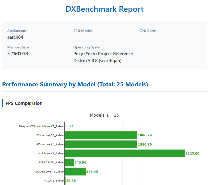
Benchmark
A benchmark tool named dxbenchmark is provided as part of the dx-rt repository. This tool can be used to quickly evaluate the inference performance of different models on the DX-M1 accelerator.
Run the following command to benchmark all models located in the assets/models directory. In this example, 100 inference loops are executed for each model:
dxbenchmark --dir assets/models/ -l 100
Depending on the number of models and the selected loop count, the benchmark may take several minutes to complete. Once finished, the benchmark results are generated in multiple formats, including:
- a JSON file
- a CSV file
- an HTML report
These reports provide detailed performance metrics for each model, such as inference time and throughput.
Below is a screenshot showing a portion of the generated HTML report (it is just an example and the values are not correct).